Abstract
It is generally
accepted that the violation of 'local realism' is a distinctive feature of
quantum systems, and it cannot be modeled by classical means. Our pilot study
shows that this is actually possible. When analyzing the emulation of
well-known 'quantum paradoxes', it turns out that the key role in their
occurrence is played by the operation of the coincidence counter, which
differently distinguishes a subset of entangled pairs from the set of all
registrations. Its operation leads to the illusion of instantaneous 'spooky action'
and 'retroactive eraser', when changing the system setting changes the settings
of statistical sampling from data collected in the past. In the light of new
thought experiments, the 'collapse' of the wave function can be interpreted in
a subjective manner, as a change in the practical attitude of the
experimenter's mind, which does not contradict however the objective nature of
reality. In this case, the wave function is only a way of describing
statistical 'ensembles' in the Blokhintsev's sense. The presence of
non-classical interference between distant macroscopic cyclic processes should
lead to non-local effects in animate and inanimate nature and in the human
brain.
Breaking 'local realism': classic emulation
Violation of
'local realism' in physics is understood as a situation in which difficulty
arises when trying to explain the results of measurements in terms of the
properties of a predetermined number of physical objects. At the same time, the
properties of physical objects should not change instantly, depending on any
remote actions. Mathematically, most often in the literature, violation of
local realism is presented in the form of violation of certain combinatorial
inequalities - Bell's inequalities. However, there is another, less abstract
and more visual way of representing the violation of 'local realism': through
the function of the dependence of the degree of correlation of the spins of two
entangled particles on the mutual directional angle of the sensors of their
registration:

Fig. 1 from Wikipedia https://en.wikipedia.org/wiki/Bell%27s_theorem#/media/File:Bell.svg
Blue graph: quantum case (with local realism
violation)
Red graph: classic (preserving local realism)
According to
general theoretical considerations, in the quantum case, the graph of this
dependence should be sinusoidal, while any case of preservation of 'local
realism' requires a linear dependence of the degree of correlation of spins on
the mutual angles of the sensors on the intervals: 1) from 0 to 180 angular
degrees and 2) from 180 to 360. This difference is reflected in Fig. 1, where
it is clearly seen that the predictions of the quantum theory coincide with the
predictions of the locally realistic theory only at the nodal points, when the
mutual angles of the sensors are 0, 90, 180, 270 and 360 °, and in other cases,
they diverge.
To get a deeper
understanding of the 'local realism' preservation or violation, we developed a
thought experiment to emulate the violation of 'local realism' by classical
means.
Let's carry out a
gedankenexperiment: imagine that in the direction of Alice and Bob, whose
laboratories are in zero gravity at a distance in space, pairs of macroscopic
disks are launched at different random angles in a certain plane (YZ). All
discs are the same size and painted the same: one side is painted red and the
other blue.
All participants
in the experiment know in advance that in each pair the disks are launched at
the same angle to the Z and Y axes, but at the same time, if we take the set of
launched pairs, the angles are randomly distributed between the pairs of disks.
However, for any pair of disks being launched, it is known that if one disk in
a pair is located with its red side in one direction, then the other is in the
strictly opposite direction.

Fig. 2
The registration
of arriving disks in each space laboratory is as follows: at the edge of a
circular hole in the plane (YZ) in the spacecraft of Alice and Bob, which are
distant from each other, through which disks move, there is a registration
sensor directed to the center of the hole. It knows how to register the red or
blue side of the discs flying through the hole. If the disc is turned towards
it with the red side at least at a small angle, the arrow sensor registers
'red', if on the contrary, then 'blue':
 Fig. 3
In Figure 3, the
registration holes in the space laboratories of Alice and Bob are superimposed
on one another. During the experiment itself, these holes are located at a
distance, in strictly parallel planes. The sensors for registering disks for
Alice and Boris are mutually located as shown in the diagram: at an angle φ.
Such an
experimental design allows us to speak of a statistical correlation between the
registration of the 'red' and 'blue' sides of the arriving disks at A. and B.
Namely: if the relative angle between the directions of the sensors A. and B.
is equal to φ, the pairs of disks with the normal directions in Sectors 8, 1,
2, 4, 5, 6, will anticorrelate, that is, if A. gets the result 'red', then B. -
'blue', and vice versa.
If the pairs of
disks have a normal direction in sectors 3 or 7, then the measurement results
will be correlated in the sense that: if A. gets the result 'red', then B. will
receive the result 'red', and if 'blue', then the partner also will have 'blue'
registered. This is despite the fact that objectively the sides with the same
color in a pair of discs are always directed in different directions.
Since the angles
of orientation of different pairs during every throw are distributed in advance
and randomly, that is radially symmetrically, the correlation probability
p(same) is determined in this experiment by the ratio of the areas of the
correlated sectors to the total area of the
circle. Since the areas of the sectors linearly depend on the angle φ in the intervals [0.90 °], [90 °, 180
°], [180 °, 270 °],
[270 °, 360 °], the probability p(same) of the correlation between
the sensor readings Alice and Bob will also linearly depend on the angle φ.
At an angle φ =
0, the areas of the correlated sectors are zero, which means that the ratio of
the anticorrelation sectors to the total number of sectors is 1, the
probability of anticorrelation is 100%, and of correlation is 0%. In other
words, at a zero angle between the direction of Alice's and Bob's detectors,
each of them with a 100% probability knows at the moment of receiving its
partner disk that if its detector registered 'red', the partner's detector
registered 'blue'. Correlation:
С = p(same) -
p(diff) = - 1.
At the angle φ =
π / 2 = 90 °, the areas of the correlating and anticorrelation sectors become
equal, which means that at the moment of obtaining the disc, each of the
experimenters can know the partner's result only with a probability of 50 to
50%: 'red' or 'blue'. In other words, with the orthogonal arrangement of the detectors,
there is no definite correlation between the readings of detectors A and B. Thus,
the correlation С = p(same) - p(diff) = 0.
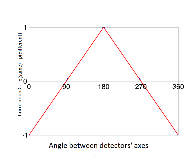
Fig. 4
At an angle φ =
π = 180 °, the areas of the anticorrelation sectors are zero, which means that
the ratio of the correlated sectors to the total number of sectors is 1, the
probability of correlation is 100%, and the probability of anticorrelation is
0%. In other words, with such an angle between the direction of Alice's and Bob's
sensors, when Alice receives the result 'red', the result of Bob will always be
'red'. Correlation degree C = p (same) - p (diff) = 1.
With further
mutual rotation of the axes of the sensors by an angle φ over 180 °, the slope
of the dependence graph at the point φ = 180 ° changes its sign, as shown above
in Fig. 4.
As you can see, such
a correlation dependence corresponds to the dependence shown in Fig. 1, which
reflects the presence of 'local realism': each triggering of the sensor
corresponds to an already available physical object with the corresponding
physical property, which is registered by the sensor.
Condition
Leading to Violation of 'Local Realism'
Let's supplement
our experiment with the following condition: not all disks will be registered,
but only with a certain probability pdet. In turn, the probability pdet
of the sensor operation will depend on the angle α between the sensor axis and
the normal to the disk the sensor observes the disk flying through the hole: pdet
= cosα.
Let p(same) be
the probability of registering correlated pairs, and p(diff), respectively,
anticorrelating ones.
1 / Let us show
that under this condition, the new ratio of the probabilities of triggering the
sensors in the anticorrelated and correlated sectors p*(diff) / p*(same) will
be greater than the corresponding ratio of probabilities p(diff) / p(same)
observed under the conditions of 'local realism'.
1-a) The ratio of the probabilities of
detection while observing 'local realism' is equal to the ratio of the areas of
the anticorrelating and correlating sectors:
p(diff) /
p(same) = S(diff) / S(same) = (ϕ + 2 (π/2 - ϕ)) / ϕ = π/ϕ - 1
Source and
meaning of violation of 'local realism' in emulation experiment
As can be seen
from the following figure, the straight lines corresponding to the mathematical
expectations of the normals in the correlated and anticorrelation sectors are
the bisectors of the sector-forming angles. Violation of 'local realism' is due
to the fact that the mathematical expectation (averaged location) of the normal
vectors of pairs of quasi-entangled disks with respect to their normals can
form different angles with the axes of two sensors, and, therefore, can lead to
different degrees of registration of correlated and anticorrelated pairs at a
certain angle ϕ
between the sensors:

Fig. 5
Mathematical expectation of normals for disk pairs in the correlated
(8,1,2,4,5,6) and the anticorrelated (7,3) sectors
1-b) Correction to the ratio of
probabilities introduced by the new condition:
αsame - is
the angle between the mathematically expected normal to the pairs of disks in
the correlated sectors and the axes of the sensors.
αdiff - is
the angle between the mathematically expected normal to the pairs of disks in
the anticorrelated sectors and the axes of the sensors.
For the angle
between the axes 0 <φ <π / 2:
cosαsame
= cos (π/2 - φ/2) = sin(φ/2)
cosαdiff
= cos(φ/2)
The correction
to the registration probability of each pair is equal to the square of the
correction to the registration probability of each disc. Total we get:
p*(diff) =
p(diff) cos2αdiff
p*(same) =
p(same) cos2αsame
p*(diff) /
p*(same) = p (diff) ⋅ cos2αdiff / (p(same) ⋅ cos2αsame) = p(diff) / {p(same) ⋅ tg2(φ/2)} ⇒
1-c ) since 0 <tg2(φ/2)
< 1, then:
p*(diff) / p*(same) > p(diff) / p(same)
over the entire interval 0 < φ < π / 2
2 ) Let us show that with the fulfillment of the
new registration condition for two-color disks, the correlation function С,
defined by us as С = p(same) – p(diff) (see Fig. 4), becomes less than it was
before (in a locally realistic situation).
2-a ) Let us express the correlation function C
through the ratio of the probabilities p(diff) / p(same) of anticorrelation and
correlation:
According to the
definition, С = p(same) - p(diff), which is equivalent to: С = p(same) -
p(diff) ⋅
p(same) / p(same) = p(same) ⋅ (1 –
p (diff ) / p(same))
According to the
definition of probability:
p(diff) +
p(same) = 1 (condition for normalizing the probability to one) ⇒
p(same) = 1 / ((p
(diff) / p (same) + 1)
We substitute
the expression 1 / ((p (diff) / p (same) + 1) instead of p(same) in the first equation, and
get:
С = (1 - p(diff)
/ p(same)) / (1 + p(diff) / p(same))
2-b ) For convenience, we denote the ratio of
probabilities as a: p(diff) / p(same)
≡ a
Then the
correlation C can be written as:
C = (1 - a) / (1
+ a)
The same values after
the fulfillment of the new disc registration condition will be denoted by an
asterisk *:
C* = (1 - a *) /
(1 + a *)
Let us show that
C* is less than C over the entire interval 0 < φ < π/2.
2-c )
From 1-c ) we know that the ratio
of the probabilities is p*(diff)
/ p*(same) > p(diff) / p(same) – over the entire interval 0 < φ < π/2 .
With the new designations,
this means that a*> a on the entire interval: 0 < φ < π / 2, which
makes it possible for us to express a* through a, as: a * = a + Δa
Now the formula
for correlation C looks like this:
C = (a - 1) / (a
+ 1)
С * = (1 - a -
Δa) / (1 + a + Δa) = – ((a + Δa) - 1) / ((a + Δa) + 1)
But for a > 1
and Δa > 0 always fulfilled: ((a + Δa) - 1) / ((a + Δa) + 1) > (a - 1) /
(a + 1)
In other words,
for a > 1 and Δa > 0 always fulfilled: |C*| > C, but since on the
entire interval 0 < φ < π/2,
both C and C * are less than 0, then:
The condition С
* < С is fulfilled over the entire
interval 0 < φ < π / 2 , as it pictured on the next figure:
 Fig. 6
Similarly, it can be shown that on the interval π/2 < φ < π of the angle between the axes of the detector, the correlation function C* with the additional condition of registering is always greater than the initial C, which was what we needed to demonstrate that in our thought experiment an emulation of local realism violation occurs:
 Fig. 7
General
conclusions from emulating violation of 'local realism'
This emulation
demonstrates that it is not necessary for physical properties to occur at the
time of registration to violate 'local realism' and Bell's inequalities. It is
enough that the detection of physical reality does not occur ideally, but with
some systematic losses depending on the conditions of the experiment. In this
case, with the consistent application of Bohr's approach to the interpretation of
the results of experiments, one should abstract from unrecorded reality, as
from a 'thing-in-itself', and speak only about the statistics of a series of
experiments, and its 'objective laws'. At the same time, it is absolutely not
necessary that the 'objective reality', which is not captured in the
experiment, should be absent in principle.
If we adhere to
Einstein's approach to objective reality, as something independent of
measurements, we can interpret the results of emulation as a model with 'hidden
parameters', which are the phases of rotation of the discs being thrown. But
even in this case, the possibility of particle-wave emulation of 'spooky action
at a distance' shows that, contrary to what Einstein thought, not only in
quantum mechanics, but also in classical mechanics, cases of 'spooky action at
a distance' can arise, which can be fully explained by the presence a common
local cause in the past.
Emulation of
quantum interference by classical means
In the previous
chapter, in a gedankenexperiment to emulate the violation of 'local realism',
we assumed that a pair of two-color disks launched to the detectors remain
oriented in the same plane throughout their trajectory. In fact, this condition
is redundant. Suffice it to assume that, if the orientation does change, it
changes correlatedly, so that the planes of the disks remain with each other at
an angle known at any time (constant zero in the simplest case). Thus, the
discs can rotate synchronously while flying to their detectors. In the simplest
case, the discs can rotate at the same speed and still fly at the same speed.
In more complex cases, the rotation of the disks and their movement can be with
different speeds and frequencies, however, knowing the frequencies and speeds,
we can always calculate the difference in the rotation phase of the disks from
one pair, provided that we know their initial state.
Let us define,
as a 'quasi-slit', a device that, when a disk passes through it, randomly
'scatters' its trajectory within the angle θ, while maintaining its orientation
in space, linear velocity, phase and rotation frequency.
 Fig. 8
Let us assume
that the probability density of disc throwing in a certain direction within the
framework of the angle θ of quasi-diffraction by the quasi-slit is uniformly
distributed within the framework of the given angle θ.
Imagine that
pairs of disks in our experiment, before getting from the source to the detectors,
fly through two 'quasi-slits', each through its own. Let's leave only one detector,
because now it will be able to receive quasi-entangled pairs passing through
both quasi-slits. In this case, due to the scattering of the disks, the detector
will be able to register fewer pairs of disks, but the set of quasi-entangled
pairs that will be registered will be distributed nonuniformly along the X
axis.
 Fig. 9
Obviously, due
to the different length of the trajectories, the disks will fly up to the
recorder with a different rotation phase difference depending on the position
of the recorder on the X axis. Moreover, at those points of the recorder on X,
where the disks will fly at small angles of their normals to the sensor axis, quasi-interference
'ridges' will be observed, and in those where disks arrive at angles close to
90°, registration frequency 'dips' will be observed.
 Fig. 10
As in the case
of wave interference, this quasi-interference will give a stable pattern only
if the source is coherent, that is, when the initial phases and velocities of
the disks are the same for different quasi-entangled pairs. Otherwise, for
example, if the initial conditions are randomly distributed over time, a stable
interference pattern will not be observed.
If you use not
one, but two remote sensors, the interference pattern will be of the second
order or 'distant'. This 'non-classical' interference will occur when the
sensor moves along the X-axis, provided that the second sensor remains fixed as
shown in the figure 11 below and data from both detector is collected and
filtered by a coincidence counter.
 Fig. 11
For the
appearance of interference, the expansion angles α and α1 of the
disks after passing through their quasi-diffractor (quasi-diffraction slit)
should be sufficient to form a phase difference between the rotation of the
disks depending on the paths.
When changing
the settings for receiving discs for one observer, the interference pattern
will change instantly, although this pattern can be distributed at an
arbitrarily large distance from the laboratories of Alice and Bob from each
other. Moreover, this 'instant' nature of the changes will be documented by the
data of laboratory journals about the time of arrival of the quasi-entangled
partners. But the observer, before being able to draw such a conclusion, must
receive information from both detectors using the classical channel, so that
the fact of superluminal correlation cannot be interpreted as 'instantaneous
transmission of information from Alice to Bob's and used immediately. Obviously,
this happens because information about the correlation of properties between
quasi-entangled partners is not localized at one point in space, and its
arrival is distributed non-locally between two mutually distant registration
events.
In the case of second-order
quasi-interference in this experiment, the initial phases of the disks can be
randomly distributed between pairs, but quasi-entanglement of the phases of
rotation of the disks inside each pair should remain. In this case, Alice and
Bob, moving alone their detectors along the X-axis, will not detect first-order
interference, since the distribution of the initial phases in one stream is not
coherent. However, ex post facto, if coincidence counter is used, by comparing
the results of their observations in laboratory journals they will be able to
detect nonclassical second-order interference in many quasi-entangled pairs.
This is explained by the fact that the set of quasi-entangled pairs, regardless
of their initial orientation but depending on the length of their trajectories,
under the conditions of our experiment will decompose into equivalence classes
in terms of the phase difference at the time of registration. These equivalence
classes will register with different probabilities.
This result resembles
the results of quantum experiments, in which also one detector cannot detect
interference, but with a special method of connecting the results of
measurements in A and B to a coincidence sensor, interference is detected. Just
as in this emulation, in quantum experiments, interference is detected on
many pairs of particles, when information about the interference is not
localized at a point, but is distributed between remote detectors.
Heisenberg lens
emulation
Let us define
the Heisenberg quasi-lens in our emulation experiments as a device that, when a
two-color disk passes through it, regardless of the approach trajectory,
directs it to the focus point without changing the speed, phase and rotation
frequency.
 Fig. 12
Since the disk
moving towards the detector are passing through the center and the edge of the
quasi-lens, their tralectories are not equal in length. So, the coherently
oriented disks flying along these paths will experience different phases at the
time of registration. This shift will lead to quasi-interference on a set of
disks arriving at the detector along different paths, which in turn will be
noticeable when the detector moves along the X-axis from point A through point
B to point C (provided that the entire ensemble of registered pairs is coherent
in its rotation in the XY plane).
Emulation of
Zeilinger's experience
In this
experiment on nonclassical distant interference (second-order interference) of
pairs of entangled photons, a double-slit screen with a movable detector is
installed on one arm (detector B), and a Heisenberg lens on the other (detector
A). Depending on whether the detector is in the focus of the Heisenberg lens or
not, distant interference (second-order interference) appears or disappears in
the ensemble of photon pairs (Anton Zeilinger. 'Experiment and the foundations
of quantum physics').

Fig. 13 (from Zeilinger's article)
To emulate this
experiment, we will apply an experiment with a source of color-quasi-entangled
pairs of two-color disks, throwing at the same speed v towards the detectors of
Alice and Bob. The disks rotate in the XY plane of the detectors with a
constant frequency ω so
that at the same distance of two disks of the same pair from the source, their
rotation phases are the same.
For moving uniformly rotating discs, the phase
difference at the time of their registration is equal to:
Ф2 - Ф1 = - ω / v (r2 - r1)
Thus, in our
experiment, the phase difference is completely determined by the difference in
the path length from the source to the detector.
Let us define in
our experiment a classical analogue of the source of photon pairs from the
Zeilinger's experiment, designating it as a 'quasi-crystal'. In his experiment,
pairs of photons are obtained entangled in color and simultaneously in paths. That
means for each pair of photons in the general case, if the path of one partner
is known, then the path of the other is also known. A quasi-crystal in our
experience acts in a similar way: in addition to the fact that it forms pairs
that remain in the same plane during its rotation, it also distributes these
pairs randomly along different, non-intersecting paths:

Let's set up a
setup to emulate the Zeilinger's experiment using a quasi-crystal, a Heisenberg
quasi- lens, and two quasi-slits.

If the D1 sensor
is not in the focal plane of the quasi-lens, the coincidence counter selects
from the ensemble of registered pairs only those that follow the same path: 1
or 2. There can be no interference, since the phases of the disks traveling in
different paths do not add up in the counter.
If the D1 sensor
is placed in the focal plane of a quasi-lens, the coincidence counter combines
many registered pairs that follow different paths. Correspondingly, there will
be quasi-interference of a set of pairs going along paths 1 and 2, according to
the difference in their phases at two points of registration: in detectors D1
and D2.
Thus, the
appearance or disappearance of quasi-interference is associated with different
sampling made by the coincidence counter from the general ensemble of
registered pairs, at different positions of the detector D1.
Moreover, if the
path to the Heisenberg lens is significantly lengthened, a change in the
position of the D1 sensor through a change in the sample of pairs can influence
'retrospectively' our ideas about the past, leading to the illusion of
'appearance' or 'erasure' of interference in the past, that is, to the effect
of 'the quantum eraser '.
This result
shows that with a clear understanding of the role of the coincidence counter,
remote property changes are no longer a 'spooky' action. Obviously, we are
talking about information related to a common past, distributed between remote detectors,
when information received to one detector does not have an adequate semantic
interpretation, but is just a part of the 'message' or 'knowledge' received on
two detectors simultaneously .
Conclusions
regarding the 'collapse of the wave function'
The fundamental
possibility of emulating quantum experiments by classical means makes it
necessary to clarify the understanding of the 'collapse of the wave function'.
It turns out that a similar 'instantaneous collapse' of probability
distribution to a single value is not more, than a technical transition from
considering knowledge about a set of events (an ensemble of experiments) to
knowledge about a single event (registration at some point in space).
At the same
time, the old knowledge about the 'ensemble' does not disappear and does not
'collapse', it can still be used to predict new events. It simply loses its
relevance in connection with the acquisition of new knowledge and a change in
the practical attitude of the researcher. In this sense, the 'collapse' of the
probability distribution function is completely subjective and 'occurs in
consciousness', reflecting changes in the practical attitude, but this
subjectivity is by no means a denial of 'objective physical reality'. On the
contrary, there is every reason to consider the wave function itself an
objective reality in the spirit of Blokhintsev's quantum ensembles interpretation.
It is also
interesting that such an explanation of the 'collapse' of the probability
distribution function is compatible with different versions of the
interpretation of probability theory, both Bayesian and classic. After all, any
'a priori' knowledge about a set of experiments before they are carried out can
also be understood as obtained 'a posteriori' by previously conducted
experiments, that is, as an 'objective physical reality'.
Consider next
the gedankenexperiment of Wigner's friend. It raises the question: how to
understand the situation when one experimenter, who is inside the laboratory,
has already recorded the result of measuring the quantum state, and the other,
who is outside, outside the zone of access to the sensor readings, has not yet
learned about the measurement. The picture above is from Massimiliano Proietti
et all. Experimental test of local observer-independence shows a diagram of an
experiment, during which two experimenters, who are inside two closed
laboratory rooms, measure a pair of photons entangled in polarization:
 Fig. 16
Their two
colleagues do not know anything about the fact of measurement.
From the point
of view of the Copenhagen interpretation of quantum mechanics, for observers
inside who received the measurement data, the superposition of 1/√2 (| h⟩ ± | v⟩)
states h and v turned into one of four possible 'projections': hh, hv, vh, vv .
However, from the point of view of observers who do not have access to the fact
of registration of this pair of particles, the system is still in a
superposition of quantum states | h⟩ and | v⟩.
The fundamental
possibility of the classical emulation of experiments with the 'collapse of the
wave function' makes it possible to explain this situation in a different way:
if the system settings have not changed, then from any point of view, after
registering a pair of particles, the system continues to be in the
superposition 1/√2 (| h⟩ ± |
v⟩ ), understood
either as a quantum superposition or as a superposition (interference) of the
rotation phases of classical particles in an emulation experiment. The
preservation of the superposition of states is confirmed by the fact that the
statistics of subsequent measurements in the ensemble of uniform experiments
will correspond to the corresponding probability distribution in observer
independent way.
Thus, there is
no objective transition of superposition to projection, but there is - the
acquisition of new knowledge, the conditions of access to which may be objectively
different for different observers. The wave function, understood as a property
of an ensemble of experiments, is completely objective, and its 'collapse' is
completely subjective, and corresponds to a change in the practical attitude of
consciousness. It should be recognized that the results of the work of
Massimiliano Proietti et all. Experimental test of local observer-independence,
which demonstrated the preservation of the quantum superposition after the
measurement, is more consistent with the interpretation of quantum ensembles
than the Copenhagen interpretation. At the same time, the 'collapse of the wave
function' in the spirit of Mensky's interpretation should be identified with
the work of consciousness.
Update 04.04.21:
Through the efforts of A. Kaminsky, the model of
emulation of the violation of 'local realism' by classical means was tested in
a computer simulation (MATLAB program). I am grateful to A. Kaminsky for the discussion and for the provided results of the computer simulation. However, at his request I inform that he does not agree with my interpretation of the results obtained. The
main simulation results are shown in Figure 16:

When reduced to the probability norm, taking into account the operation of the coincidence counter, the ratio of the probability distribution functions in the classical case (indicated in black in Fig. 16) and in theoretical emulation (indicated in blue in Fig. 16) corresponds to the form of violation of 'local realism' (Fig. 1). If the fact that incomplete pairs are cut off by the coincidence counter was not taken into account, emulation does not lead to a violation of 'classical realism', which may indicate a significant, if not decisive, role of the coincidence detector in experiments to check the violation of 'local realism'.
Full report on computer simulation of the model by A.
Kaminsky (translated from Russian):
EPR - experiment simulation
In fig. 1 shows the result of computer simulation of an EPR type experiment.
The blue curve is the classical correlation of two
photons with the same polarization.
Red curve - a hidden parameter is enabled (see
appendix) that simulates the collapse of an entangled state.
As can be seen from the figure, the simulation result
corresponds to Bell's theorem. When the hidden parameter (entanglement
simulation) is enabled (see Appendix: hidden parameter h1), the correlation in
the entire range of angles exceeds the classical Bell's threshold.

Fig. 1
The result is completely identical to that given in
[1]
Bi-Colored Disk model simulation
The following fig. 2 shows the result of computer
simulation of a model of rotating disks (I. Dzhadan). Similar models were
discussed here [2]
The blue curve is the classic Bell correlation (linear
versus angle).
Red curve - corresponds to the correlation with
artificially introduced losses. Moreover, the probability of losses ('quantum
efficiency') depends (as the square of the cosine) on the angle between the
polarization (the angle of rotation of the disk) and the angle of the detector.
Correlation was normalized to the total number of events.
As can be seen from the figure, the magnitude of the
correlation in the entire range of angles turns out to be less than the
limiting value for the classical models. That is, the simulation result
corresponds to Bell's theorem.

Fig. 2
Figure 3 shows the simulation result, which differs from the previous one only in that, under loss conditions, when calculating the correlation, events without loss of photons (blue curve) were taken into account, as well as the case when the loss of 1 photon was allowed (red curve).
It can be seen that the first case (when events are
taken into account by the coincidence counter) violates Bell's inequalities,
while the second case (the loss of at most one photon) fits into the framework
of classical behavior (Bell's inequalities are not violated).

Fig.3
Literature:
2. https://www.mdpi.com/1099-4300/22/3/287
Appendix (Programs in matlab)
Monte Carlo computer program for EPR experiment
simulation
% --- Main Experiment protocol --------
clear all;
N=500; %trials
M=180; % angles
f1=90*2*pi/360;
for j=1:M
f=j*2*pi/360;
[Y1,Y2] = Source2(N);
A(j)=f;
[Alice,h1] =
Registration2(Y1,f);
Y2=h1; % hidden
parameter (uncomment if need)
[Bob,h2] =
Registration2(Y2,f1);
CORR(j)=sum(Alice.*Bob)/N;
disp(j);
end;
plot(360*A/(2*pi),CORR);% hold on; plot(360*(A-1)/NN,CORRZ);
hold on;
function [Y1,Y2] = Source(N)
% N- number of trials
Y1=2*pi*rand(1,N);
Y2=Y1;
function [pol,h] = Registration(Y,A)
%Y=Y1;
% Y(:) - photons polarizations
% A - detector angle
N= numel(Y);
%------------------------
p=(cos(A-Y)).^2;
population = 0:1;
sample_size = 1;
for k=1:N
pmf = [p(k), 1-p(k)];
s=randsample(population,sample_size,true,pmf);
pol(k) =(-1)^(1+s);
if pol(k)==-1
h(k)=A;
elseif pol(k)==1
h(k)=A+pi/2;
end;
Monte Carlo computer program for Bi-Coloured Disk model simulation
% --- Main Experiment protocol --------
clear all;
NN=100;
MM=1000;
Y = Source(NN,MM);
Y1=Y; Y2 =
circshift(Y1,[NN/2,0]);
for i=1:NN
A(i)=i;
[Alice_meas,Alice_Meas_bitZ] =
Registration(Y1,A(i),NN,MM);
B=1;
[Bob_meas,Bob_Meas_bitZ] = Registration(Y2,B,NN,MM);
CORRZ(A(i))=sum(Alice_Meas_bitZ.*Bob_Meas_bitZ)/MM;
S1=sum(abs(Alice_meas.*Bob_meas)); % loss of 1 or 2
photons
S2=sum(sign(abs(Alice_meas)+abs(Bob_meas))); % loss of
2 photons
CORR1(A(i))=sum((abs(Alice_meas.*Bob_meas)).*Alice_meas.*Bob_meas)/S1;
CORR2(A(i))=sum((sign(abs(Alice_meas)+abs(Bob_meas))).*Alice_meas.*Bob_meas)/S2;
end;
plot(360*(A-1)/NN,CORR1,'b'); hold on; plot(360*(A-1)/NN,CORR2,'r');
plot(360*(A-1)/NN,CORRZ,'k');
function Y = Source(N,M)
% N- number of angles
% M- number of particles
D=[-1*ones(N/2,1);ones(N/2,1)];
for i=1:M;
r = randi(N);
Y(:,i) = circshift(D,[r,0]);
A(i)=r;
end;
function [Meas_bit,Meas_bitZ] = Registration(Y,A,NN,MM)
% Y(:,:) - photon discs
% A - detector angle
% NN - number of angles
% MM - number of trials
%------------------------
bit=Y(A,:);
%-----------------------
%Find Angle
[Alpha] = FindAngle(Y,NN,MM);
% Correction
for k=1:MM
p=(([cos(2*pi*(A-Alpha(k))/NN)]^2))*1;
pmf = [p, 1-p];
population = 0:1;
sample_size = 1;
correction_random_bit(k) = randsample(population,sample_size,true,pmf);
end;
%-----------------------
Meas_bit=correction_random_bit.*bit;
Meas_bitZ=bit;


Call me crazy, but the title of this forum Defunct Humanity never really bothered me when you were talking about Russian military stuff... but talking about complex maths and high level physics it seems to take on a more sinister tone... :)
ReplyDeleteI went through a very painful breakup with my boyfriend. We stopped talking, and he even blocked me on all social media. I was heartbroken and didn’t know what to do, so I started searching online for help. That’s when I came across several testimonies about Dr. Dawn and how he had helped people reunite broken relationships and marriages, as well as helped women conceive through his guidance.
ReplyDeleteAt first, I was unsure, but I decided to reach out to him. When we spoke, he told me things about myself and my relationship that were surprisingly accurate. He then guided me on what I should do.
To my surprise, within 48 hours, my boyfriend—who had completely cut me off—started calling me and sending me many messages, apologizing and asking for forgiveness. I forgave him, and we got back together.
Not only that, but with his support and guidance, we are now blessed with two beautiful children.
I am truly grateful for everything, and I strongly recommend Dr. Dawn to anyone going through relationship, marriage, or fertility challenges.
His WhatsApp : +2347041196471
dawnacuna314@gmail.com